Wannier90 wout file

This example shows how to plot the convergence of the wannierization cycle using the .wout file produced by wannier90. Use abiopen FILE.wout for a command line interface and the –expose option to generate matplotlib figures automatically.

• 
• 

================================= File Info =================================
Name: example01_gaas.wout
Directory: /home/runner/work/abipy/abipy/abipy/data/refs/wannier90
Size: 31.64 kB
Access Time: Thu Nov 21 11:15:55 2024
Modification Time: Thu Nov 21 11:11:43 2024
Change Time: Thu Nov 21 11:11:43 2024

================================= Structure =================================
Full Formula (Ga1 As1)
Reduced Formula: GaAs
abc   :   4.016499   4.016499   4.016499
angles:  60.000000  60.000000  60.000000
pbc   :       True       True       True
Sites (2)
  #  SP       a     b     c
---  ----  ----  ----  ----
  0  Ga    0     0     0
  1  As    0.25  0.25  0.25

Wannier90 version: 2.1.0+git
Number of Wannier functions: 4
K-grid: [2 2 2]

================================= WANNIERISE =================================
 iter  delta_spread  rms_gradient   spread  time     O_D     O_OD    O_TOT
    0  4.470000e+00  0.000000e+00 4.468812  0.00 0.00832 0.503629 4.468812
    1 -1.930000e-03  6.679013e-02 4.466881  0.00 0.00803 0.501988 4.466881
    2 -8.930000e-10  4.544940e-05 4.466881  0.01 0.00803 0.501988 4.466881
    3  0.000000e+00  2.000000e-10 4.466881  0.01 0.00803 0.501988 4.466881
    4  8.880000e-16  2.000000e-10 4.466881  0.01 0.00803 0.501988 4.466881
   16 -8.880000e-16  0.000000e+00 4.466881  0.02 0.00803 0.501988 4.466881
   17  8.880000e-16  0.000000e+00 4.466881  0.02 0.00803 0.501988 4.466881
   18  0.000000e+00  0.000000e+00 4.466881  0.02 0.00803 0.501988 4.466881
   19  8.880000e-16  0.000000e+00 4.466881  0.02 0.00803 0.501988 4.466881
   20  0.000000e+00  0.000000e+00 4.466881  0.02 0.00803 0.501988 4.466881

import os
import abipy.data as abidata

from abipy.abilab import abiopen

# Open the wout file
filepath = os.path.join(abidata.dirpath, "refs", "wannier90", "example01_gaas.wout")
wout = abiopen(filepath)
print(wout)

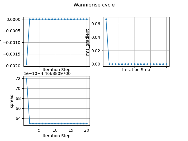
# Plot the convergence of the Wannierise cycle.
wout.plot(title="Wannierise cycle")

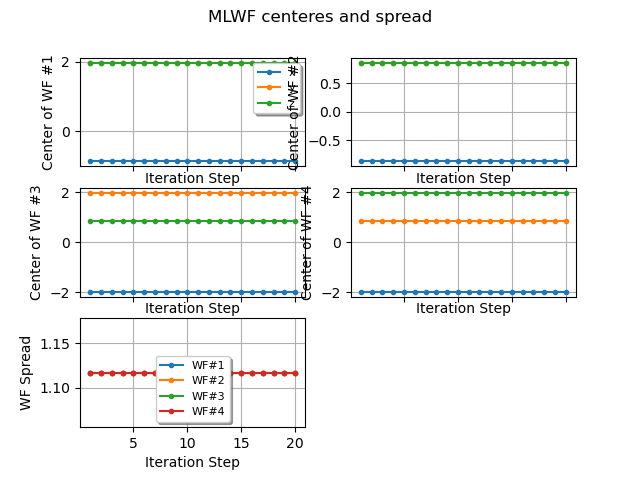
# Plot the convergence of the Wannier centers and spread
# as function of iteration number
wout.plot_centers_spread(title="MLWF centeres and spread")