Wavefunction file

This example shows how to analyze the wavefunctions stored in the WFK.nc file.

• 
• 

Out:

================================= File Info =================================
Name: si_nscf_WFK.nc
Directory: /Users/gmatteo/git_repos/abipy/abipy/data/refs/si_ebands
Size: 389.84 kb
Access Time: Wed Mar 20 21:31:02 2019
Modification Time: Wed Mar 20 16:53:35 2019
Change Time: Wed Mar 20 16:53:35 2019

================================= Structure =================================
Full Formula (Si2)
Reduced Formula: Si
abc   :   3.866975   3.866975   3.866975
angles:  60.000000  60.000000  60.000000
Sites (2)
  #  SP       a     b     c
---  ----  ----  ----  ----
  0  Si    0     0     0
  1  Si    0.25  0.25  0.25

Abinit Spacegroup: spgid: 0, num_spatial_symmetries: 48, has_timerev: True, symmorphic: True
============================== Electronic Bands ==============================
Number of electrons: 8.0, Fermi level: 5.598 (eV)
nsppol: 1, nkpt: 14, mband: 8, nspinor: 1, nspden: 1
smearing scheme: none (occopt 1), tsmear_eV: 0.272
Direct gap:
    Energy: 2.532 (eV)
    Initial state: spin: 0, kpt: [+0.000, +0.000, +0.000], name: $\Gamma$, weight: 0.000, band: 3, eig: 5.598, occ: 2.000
    Final state:   spin: 0, kpt: [+0.000, +0.000, +0.000], name: $\Gamma$, weight: 0.000, band: 4, eig: 8.130, occ: 0.000
Fundamental gap:
    Energy: 0.524 (eV)
    Initial state: spin: 0, kpt: [+0.000, +0.000, +0.000], name: $\Gamma$, weight: 0.000, band: 3, eig: 5.598, occ: 2.000
    Final state:   spin: 0, kpt: [+0.000, +0.429, +0.429], weight: 0.000, band: 4, eig: 6.123, occ: 0.000
Bandwidth: 11.856 (eV)
Valence maximum located at:
    spin: 0, kpt: [+0.000, +0.000, +0.000], name: $\Gamma$, weight: 0.000, band: 3, eig: 5.598, occ: 2.000
Conduction minimum located at:
    spin: 0, kpt: [+0.000, +0.429, +0.429], weight: 0.000, band: 4, eig: 6.123, occ: 0.000

TIP: Call set_fermie_to_vbm() to set the Fermi level to the VBM if this is a non-magnetic semiconductor

PWWaveFunction: nspinor: 1, spin: 0, band: 0
<class 'abipy.core.gsphere.GSphere'>: kpoint: [+0.500, +0.000, +0.000], name: L, weight: 0.000, ecut: 6.000000, npw: 180, istwfk: 1
Mesh3D: nx=18, ny=18, nz=18

from abipy.abilab import abiopen
import abipy.data as abidata

# Open the DEN.nc file
ncfile = abiopen(abidata.ref_file("si_nscf_WFK.nc"))
print(ncfile)

# The DEN file has a `Structure` an `ElectronBands` object and wavefunctions.
#print(ncfile.structure)

# To plot the KS eigenvalues.
#ncfile.ebands.plot()

# Extract the wavefunction for the first spin, the first band and k=[0.5, 0, 0]
wave = ncfile.get_wave(spin=0, kpoint=[0.5, 0, 0], band=0)
print(wave)

# This is equivalent to
#wave = ncfile.get_wave(spin=0, kpoint=0, band=0)
# because [0.5, 0, 0] is the first k-point in the WFK file

# To visualize the total charge wih vesta
#visu = wave.visualize_ur2("vesta"); visu()

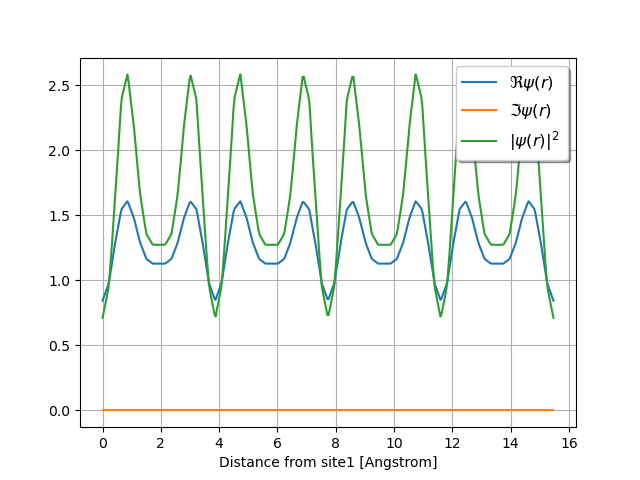
# To plot the wavefunction along the line connecting
# the first and the second in the structure:
#wave.plot_line(point1=0, point2=1)

#wave.plot_line(point1=0, point2=1, with_krphase=True)

# alternatively, one can define the line in terms of two points
# in fractional coordinates:
wave.plot_line(point1=[0, 0, 0], point2=[0, 4, 0], with_krphase=False, num=400)
wave.plot_line(point1=[0, 0, 0], point2=[0, 4, 0], with_krphase=True, num=400)

# To plot the wavefunction along the lines connect the firt atom in the structure
# and all the neighbors within a sphere of radius 3 Angstrom:
#wave.plot_line_neighbors(site_index=0, radius=3)

ncfile.close()