Ground-state SCF cycle

This example shows how to plot the results of the GS self-consistent cycle reported in the main output file.

from abipy.abilab import abiopen
import abipy.data as abidata

# Open the output file with GS calculation (Note the .abo extension).
# Alternatively, one can use `abiopen.py run.abo -nb`
# to generate a jupyter notebook.
abo = abiopen(abidata.ref_file("refs/si_ebands/run.abo"))

# Plot all SCF-GS sections found in the output file.
# Use abo.next_d2de_scf_cycle() for DFPT cycles.
scf_cycle = abo.next_gs_scf_cycle()
if scf_cycle is not None:
    scf_cycle.plot()

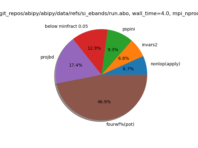
# If timopt -1, we can extract the timing and plot the data.
timer = abo.get_timer()
timer.plot_pie()

abo.close()