Density

This example shows how to analyze the electronic density stored in the DEN.nc file.

from abipy.abilab import abiopen
import abipy.data as abidata

# Open the DEN.nc file
ncfile = abiopen(abidata.ref_file("si_DEN.nc"))

# The DEN file has a `Density`, a `Structure` and an `ElectronBands` object
print(ncfile.structure)

Out:

Full Formula (Si2)
Reduced Formula: Si
abc   :   3.866975   3.866975   3.866975
angles:  60.000000  60.000000  60.000000
Sites (2)
  #  SP       a     b     c
---  ----  ----  ----  ----
  0  Si    0     0     0
  1  Si    0.25  0.25  0.25

Abinit Spacegroup: spgid: 227, num_spatial_symmetries: 48, has_timerev: True, symmorphic: True

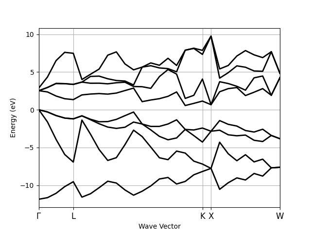
To plot the KS eigenvalues.

ncfile.ebands.plot()

density = ncfile.density
print(density)

# To visualize the total charge wih vesta
#visu = density.visualize("vesta"); visu()

Out:

Density: nspinor: 1, nsppol: 1, nspden: 1
Mesh3D: nx=18, ny=18, nz=18

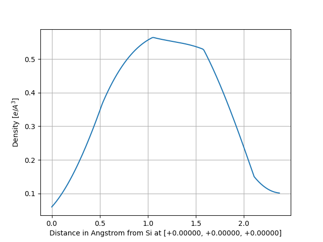
To plot the density along the line connecting the first and the second in the structure:

density.plot_line(point1=0, point2=1)

Out:

<Figure size 640x480 with 1 Axes>

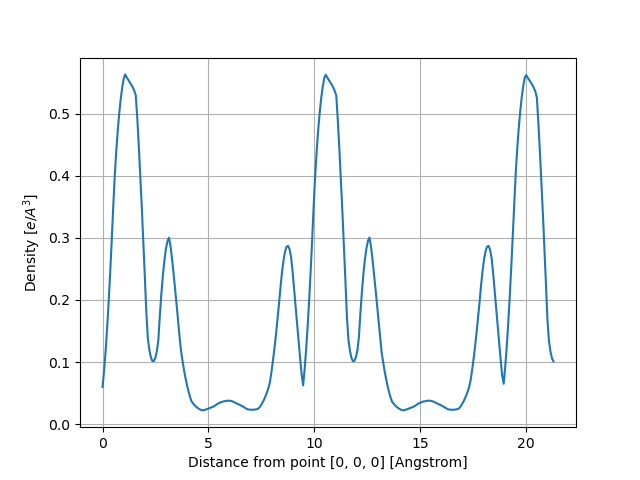
alternatively, one can define the line in terms of two points in fractional coordinates:

density.plot_line(point1=[0, 0, 0], point2=[2.25, 2.25, 2.25], num=300)

Out:

<Figure size 640x480 with 1 Axes>

To plot the density along the lines connect the firt atom in the structure and all the neighbors within a sphere of radius 3 Angstrom:

density.plot_line_neighbors(site_index=0, radius=3)

Out:

<Figure size 640x480 with 4 Axes>