MgB2 fatbands

This example shows how to plot the L-projected fatbands of MgB2 using the FATBANDS.nc files produced by abinit with prtdos 3. See also PhysRevLett.86.4656

Open the file (alternatively one can use the shell and abiopen.py FILE -nb to open the file in a jupyter notebook) Note that this file has been produced on a k-path so it’s not suitable for DOS calculations.

import abipy.abilab as abilab
import abipy.data as abidata

fbnc_kpath = abilab.abiopen(abidata.ref_file("mgb2_kpath_FATBANDS.nc"))

# To customize the matplotlib marker and its size, use:
fbnc_kpath.marker_spin = {0: "o", 1: "v"}
fbnc_kpath.marker_size = 2

Print file info (dimensions, variables …) Note that prtdos = 3, so LM decomposition is not available.

print(fbnc_kpath)

================================= File Info =================================
Name: mgb2_kpath_FATBANDS.nc
Directory: /home/runner/work/abipy/abipy/abipy/data/refs/mgb2_fatbands
Size: 149.01 kB
Access Time: Thu Nov 21 11:14:45 2024
Modification Time: Thu Nov 21 11:11:43 2024
Change Time: Thu Nov 21 11:11:43 2024

================================= Structure =================================
Full Formula (Mg1 B2)
Reduced Formula: MgB2
abc   :   3.086000   3.086000   3.523000
angles:  90.000000  90.000000 120.000000
pbc   :       True       True       True
Sites (3)
  #  SP           a         b    c
---  ----  --------  --------  ---
  0  Mg    0         0         0
  1  B     0.333333  0.666667  0.5
  2  B     0.666667  0.333333  0.5

Abinit Spacegroup: spgid: 191, num_spatial_symmetries: 24, has_timerev: True, symmorphic: False

============================== Electronic Bands ==============================
================================= Structure =================================
Full Formula (Mg1 B2)
Reduced Formula: MgB2
abc   :   3.086000   3.086000   3.523000
angles:  90.000000  90.000000 120.000000
pbc   :       True       True       True
Sites (3)
  #  SP           a         b    c
---  ----  --------  --------  ---
  0  Mg    0         0         0
  1  B     0.333333  0.666667  0.5
  2  B     0.666667  0.333333  0.5

Abinit Spacegroup: spgid: 191, num_spatial_symmetries: 24, has_timerev: True, symmorphic: False

Number of electrons: 8.0, Fermi level: 8.700 (eV)
nsppol: 1, nkpt: 78, mband: 8, nspinor: 1, nspden: 1
smearing scheme: none (occopt 1), tsmear_eV: 0.272, tsmear Kelvin: 3157.7
Direct gap:
    Energy: 0.595 (eV)
    Initial state: spin: 0, kpt: [+0.350, +0.300, +0.000], band: 3, eig: 8.402, occ: 2.000
    Final state:   spin: 0, kpt: [+0.350, +0.300, +0.000], band: 4, eig: 8.997, occ: 0.000
Fundamental gap:
    Energy: 0.058 (eV)
    Initial state: spin: 0, kpt: K [+0.333, +0.333, +0.000], band: 4, eig: 8.700, occ: 0.000
    Final state:   spin: 0, kpt: [+0.147, +0.000, +0.000], band: 4, eig: 8.758, occ: 0.000
Bandwidth: 14.314 (eV)
Valence maximum located at kpt index 27:
    spin: 0, kpt: K [+0.333, +0.333, +0.000], band: 4, eig: 8.700, occ: 0.000
Conduction minimum located at kpt index 5:
    spin: 0, kpt: [+0.147, +0.000, +0.000], band: 4, eig: 8.758, occ: 0.000

TIP: Use `--verbose` to print k-point coordinates with more digits

=============================== Fatbands Info ===============================
prtdos: 3, prtdosm: 0, mbesslang: 5, pawprtdos: 0, usepaw: 0
nsppol: 1, nkpt: 78, mband: 8

  Idx  Symbol    Reduced_Coords             Lmax    Ratsph [Bohr]  Has_Atom
-----  --------  -----------------------  ------  ---------------  ----------
    0  Mg        0.00000 0.00000 0.00000       4                2  Yes
    1  B         0.33333 0.66667 0.50000       4                2  Yes
    2  B         0.66667 0.33333 0.50000       4                2  Yes

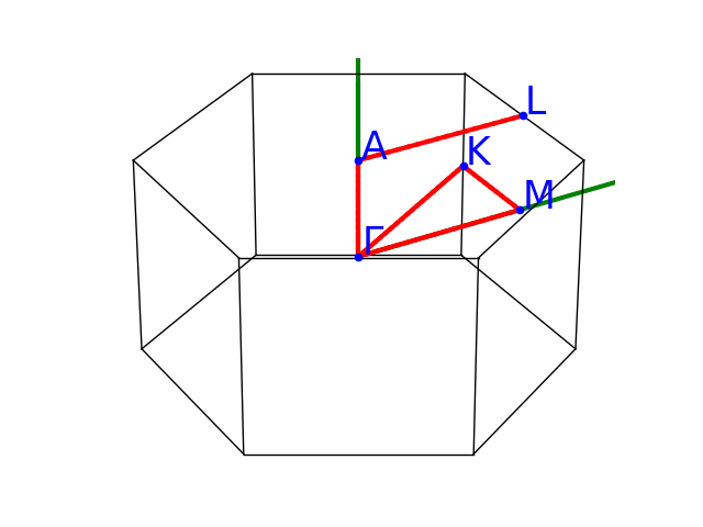
Plot the k-points belonging to the path. fbnc_kpath.ebands.kpoints.plotly()

NC files have contributions up to L=4 (g channel) but here we are intererested in s,p,d terms only so we use the optional argument lmax

lmax = 2

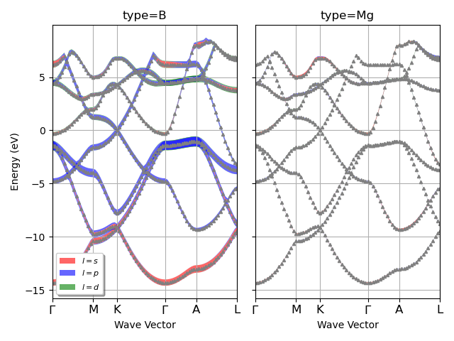
Plot the electronic fatbands grouped by atomic type. Can use l_list to select only particular l-values

fbnc_kpath.plot_fatbands_typeview(lmax=lmax, tight_layout=True, l_list=None)

For the plotly version use:

#fbnc_kpath.plotly_fatbands_typeview(lmax=lmax)

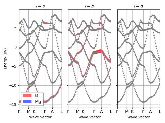
Plot the electronic fatbands grouped by L.

#fbnc_kpath.plot_fatbands_lview(lmax=lmax, tight_layout=True)

For the plotly version use:

#fbnc_kpath.plotly_fatbands_lview(lmax=lmax)

Now we read another FATBANDS file produced on a 18x18x18 k-mesh This file can be used to plot the projected-DOS

fbnc_kmesh = abilab.abiopen(abidata.ref_file("mgb2_kmesh181818_FATBANDS.nc"))

Let’s print the object

print(fbnc_kmesh)
#fbnc_kmesh.ebands.kpoints.plot()

================================= File Info =================================
Name: mgb2_kmesh181818_FATBANDS.nc
Directory: /home/runner/work/abipy/abipy/abipy/data/refs/mgb2_fatbands
Size: 480.70 kB
Access Time: Thu Nov 21 11:14:46 2024
Modification Time: Thu Nov 21 11:11:43 2024
Change Time: Thu Nov 21 11:11:43 2024

================================= Structure =================================
Full Formula (Mg1 B2)
Reduced Formula: MgB2
abc   :   3.086000   3.086000   3.523000
angles:  90.000000  90.000000 120.000000
pbc   :       True       True       True
Sites (3)
  #  SP           a         b    c
---  ----  --------  --------  ---
  0  Mg    0         0         0
  1  B     0.333333  0.666667  0.5
  2  B     0.666667  0.333333  0.5

Abinit Spacegroup: spgid: 191, num_spatial_symmetries: 24, has_timerev: True, symmorphic: False

============================== Electronic Bands ==============================
================================= Structure =================================
Full Formula (Mg1 B2)
Reduced Formula: MgB2
abc   :   3.086000   3.086000   3.523000
angles:  90.000000  90.000000 120.000000
pbc   :       True       True       True
Sites (3)
  #  SP           a         b    c
---  ----  --------  --------  ---
  0  Mg    0         0         0
  1  B     0.333333  0.666667  0.5
  2  B     0.666667  0.333333  0.5

Abinit Spacegroup: spgid: 191, num_spatial_symmetries: 24, has_timerev: True, symmorphic: False

Number of electrons: 8.0, Fermi level: 6.851 (eV)
nsppol: 1, nkpt: 370, mband: 8, nspinor: 1, nspden: 1
smearing scheme: cold smearing of N. Marzari with minimization of the bump (occopt 4), tsmear_eV: 0.816, tsmear Kelvin: 9473.2

=============================== Fatbands Info ===============================
prtdos: 3, prtdosm: 0, mbesslang: 5, pawprtdos: 0, usepaw: 0
nsppol: 1, nkpt: 370, mband: 8

  Idx  Symbol    Reduced_Coords             Lmax    Ratsph [Bohr]  Has_Atom
-----  --------  -----------------------  ------  ---------------  ----------
    0  Mg        0.00000 0.00000 0.00000       4                2  Yes
    1  B         0.33333 0.66667 0.50000       4                2  Yes
    2  B         0.66667 0.33333 0.50000       4                2  Yes

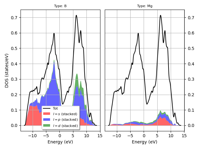
Plot the L-PJDOS grouped by atomic type.

fbnc_kmesh.plot_pjdos_typeview(lmax=lmax, tight_layout=True)

For the plotly version use:

fbnc_kmesh.plotly_pjdos_typeview(lmax=lmax)

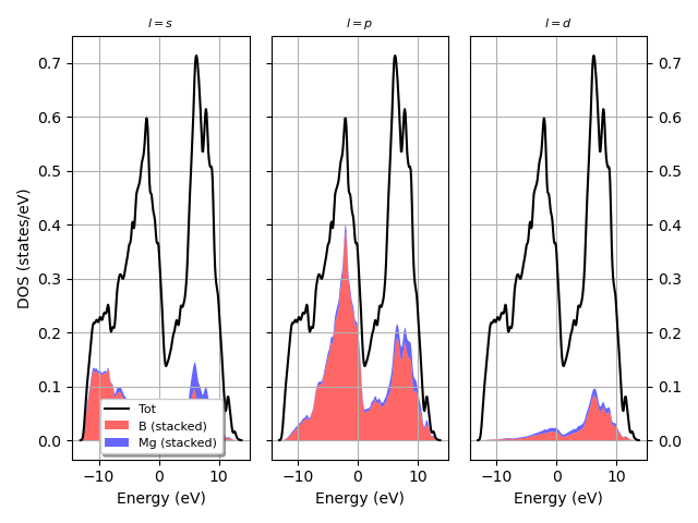
Plot the L-PJDOS grouped by L.

fbnc_kmesh.plot_pjdos_lview(lmax=lmax, tight_layout=True)

For the plotly version use:

fbnc_kmesh.plotly_pjdos_lview(lmax=lmax)

Now we use the two netcdf files to produce plots with fatbands + PJDOSEs. The data for the DOS is taken from pjdosfile. sphinx_gallery_thumbnail_number = 6

fbnc_kpath.plot_fatbands_with_pjdos(pjdosfile=fbnc_kmesh,
                                    lmax=lmax, view="type", tight_layout=True)

For the plotly version use:

fbnc_kpath.plotly_fatbands_with_pjdos(pjdosfile=fbnc_kmesh,
                                      lmax=lmax, view="type")

fatbands + PJDOS grouped by L

fbnc_kpath.plot_fatbands_with_pjdos(pjdosfile=fbnc_kmesh,
                                    lmax=lmax, view="lview", tight_layout=True)

For the plotly version use:

fbnc_kpath.plotly_fatbands_with_pjdos(pjdosfile=fbnc_kmesh,
                                      lmax=lmax, view="lview")

#fbnc_kpath.close()
#fbnc_kmesh.close()