GW with scissors operator

This example shows how to generate an energy-dependent scissors operator by fitting the GW corrections as function of the KS eigenvalues. We then use the scissors operator to correct the KS band structure computed on a high symmetry k-path. Finally, the LDA and the QPState band structure are plotted with matplotlib.

• 
• 
• 
• 

Out:

KS fermie 5.598313017568332 eV --> QP fermie 5.40710713209731 eV Delta(QP-KS)= -0.1912058854710219 eV
KS fermie 5.598453325290463 eV --> QP fermie 5.407251265916601 eV Delta(QP-KS)= -0.19120205937386192 eV

import abipy.data as abidata
from abipy.abilab import abiopen, ElectronBandsPlotter

# Get the QP results from the SIGRES.nc database.
sigma_file = abiopen(abidata.ref_file("si_g0w0ppm_nband30_SIGRES.nc"))

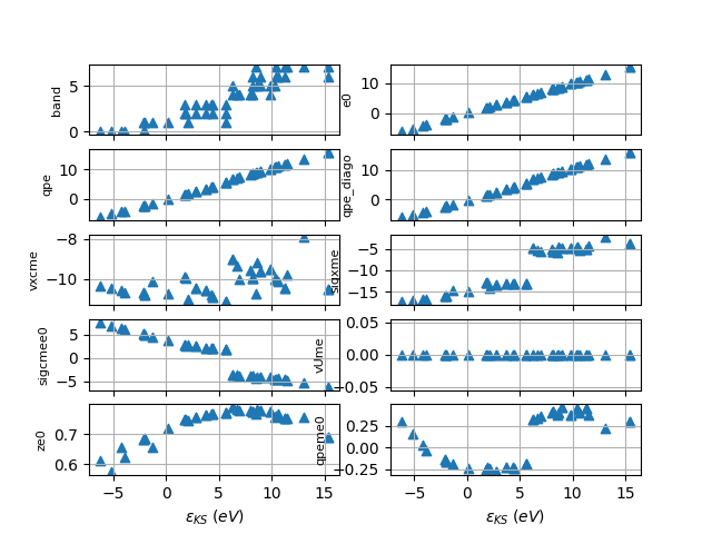
# Let's have a look at the QP correction as function of the KS energy.
# Don't shift KS eigenvalues to have zero energy at the Fermi energy.
# because we need the absolute values for the fit.
# The qpeme0(e0) curve consists of two branches:
#   the one in the [-6, 5.7] eV interval associated to valence states
#   and the one in the [6.1, 15] eV interval associated to conduction bands.
# We will fit these results with 2 functions defined in these two domains.
sigma_file.plot_qps_vs_e0(e0=None)
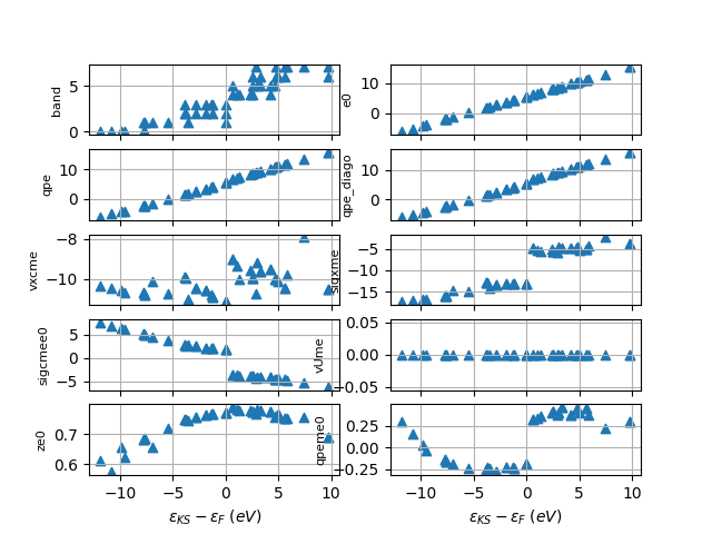
sigma_file.plot_qps_vs_e0()

qplist_spin = sigma_file.qplist_spin

# Define the two domains and construct the scissors operator
domains = [[-10, 6.1], [6.1, 18]]
scissors = qplist_spin[0].build_scissors(domains, bounds=None)

# Read the KS band energies computed on the k-path
ks_bands = abiopen(abidata.ref_file("si_nscf_GSR.nc")).ebands

# Read the KS band energies computed on the Monkhorst-Pack (MP) mesh
# and compute the DOS with the Gaussian method
ks_mpbands = abiopen(abidata.ref_file("si_scf_GSR.nc")).ebands
ks_edos = ks_mpbands.get_edos()

# Apply the scissors operator first on the KS band structure
# along the k-path then on the energies computed with the MP mesh.
qp_bands = ks_bands.apply_scissors(scissors)

qp_mpbands = ks_mpbands.apply_scissors(scissors)

# Compute the DOS with the modified QPState energies.
qp_edos = qp_mpbands.get_edos()

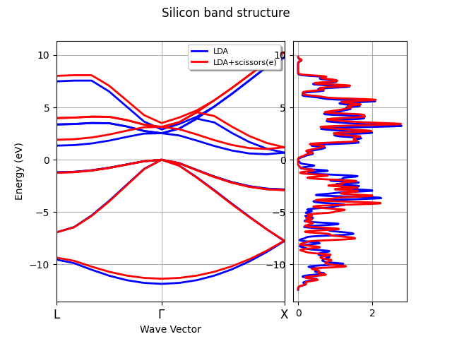
# Plot the LDA and the QPState band structure with matplotlib.
plotter = ElectronBandsPlotter()

plotter.add_ebands("LDA", ks_bands, edos=ks_edos)
plotter.add_ebands("LDA+scissors(e)", qp_bands, edos=qp_edos)

# By default, the two band energies are shifted wrt to *their* fermi level.
# Use e=0 if you don't want to shift the eigenvalus
# so that it's possible to visualize the QP corrections.
plotter.combiplot(title="Silicon band structure")

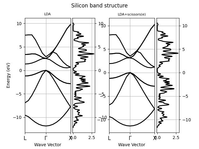
plotter.gridplot(title="Silicon band structure")
sigma_file.close()