SCR matrix

This examples shows how to plot the matrix elements of the inverse dielectric function stored in the SCR file (optdriver 3) See also plot_scr.py for the optical spectrum.

• 
• 
• 

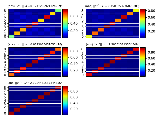
======================== inverse_dielectric_function ========================
  K-point: [+0.500, +0.000, +0.000]
  Number of G-vectors: 9
  Total number of frequencies: 35 (real: 30, imaginary: 5)
  Real frequencies up to 0.73 (eV)
  Imaginary frequencies up to 2.69 (eV)

import abipy.data as abidata
from abipy.abilab import abiopen

with abiopen(abidata.ref_file("sio2_SCR.nc")) as ncfile:
    #print(ncfile)
    # The SCR file contains a structure and electron bands in the IBZ.
    # We can thus use the ebands object to plot bands + DOS.
    #ncfile.ebands.plot()

    # Read e^{-1}_{G1, G2}(k, omega)

    kpoint = [0.5, 0, 0]
    em1 = ncfile.reader.read_wggmat(kpoint)
    print(em1)

    gvec1 = [1, 0, 0]
    gvec2 = [-1, 0, 0]

    # Plot matrix element as function of frequency along the real axis
    em1.plot_freq(gvec1=gvec1, gvec2=gvec2, waxis="real")

    # Plot data along the imaginary axis
    # Note that gvectors can also be specifined in terms of their index.
    em1.plot_freq(gvec1=0, gvec2=0, waxis="imag")

    # Plot e^{-1}_{G1, G2} along the imaginary axis.
    em1.plot_gg(wpos="imag")